You can download the challenge files and solutions here: MCTF2026-DevilDiagram-main.zip
Description (Player Facing)
Subject: Evidence Item #4B - "The St. Jude's Tapes" Background: St. Jude’s Asylum was shuttered in 1988 after the "incident" in the basement ward. Last night, urban explorers found an old medical XY-plotter plugged into a dead outlet. It was moving on its own. They recorded the sound of the machine screeching in the dark. It seems to be trying to draw something. Objective: Decipher the audio to see what the machine drew.
Solution
Step 1: Initial Reconnaissance
The player opens evidence_4b.wav in an audio editor (e.g., Sonic Visualizer or Audacity).
- First observation: It is a Stereo file. The left and right ears hear different patterns. This suggests independent data streams for two channels (Likely X and Y coordinates).

Step 2: Spectral Analysis
The player switches to a Spectrogram View. (Here we can see the two channels)
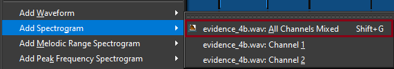
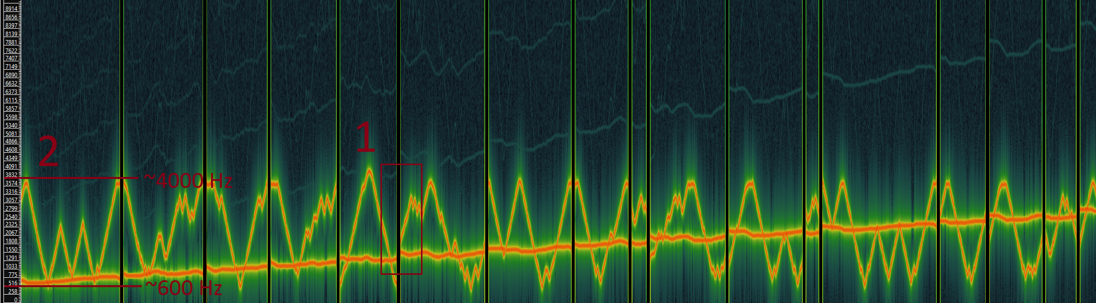
- Visual: We see a continuous stream of varying pitches, but crucially, the signal is Frequency Modulated (FM). The lines move up and down in frequency over time.
- First observation: The frequencies bounce between a specific range (600 Hz to 4000 Hz). (1)
- Second observation: There are occasional vertical gaps (silence) where the signal drops out completely. (2)
Deduction: This is an analog vector drawing.
Left Channel = X-Axis Position (mapped to pitch)
Right Channel = Y-Axis Position (mapped to pitch)
Pitch: Low Pitch = 0% Coordinate, High Pitch = 100% Coordinate.
Silence: Pen Up (Stop drawing).
Deduction 1: The machine is clearly writing text, as the movement from left to right matches typical text writing direction.
Deduction 2: The presence of gaps or silence indicates the machine is starting a new letter each time.
Step 3: Developing the Decoder
The player realizes they cannot decode this manually. They write a script to:
- Read the WAV file.
# 1. Load the file
rate, data = wavfile.read("challenge/evidence_4b.wav")- Demodulate the Signal: Use the Hilbert Transform to extract the Instantaneous Frequency (pitch) of both channels.
# 2. Extract Signal (Hilbert Transform)
analytic_x = hilbert(data[:, 0])
analytic_y = hilbert(data[:, 1])

# Calculate frequency: frequency is the rate of change of the phase
freq_x = np.diff(np.unwrap(np.angle(analytic_x)))
freq_y = np.diff(np.unwrap(np.angle(analytic_y)))- Detect Pen Lifts (Filter Silence): If the volume drops below a threshold, stop drawing.
# 3. Filter Silence (Simple "Pen Up" check)
# Only draw when the volume is loud enough (10% of max volume)
amplitude = np.abs(analytic_x[1:])  # Match length with freq array (which is one shorter)
mask = amplitude > (np.max(amplitude) * 0.1)- Plot: Draw the extracted (X, Y) coordinates. Note: We skip manual normalization here because the Plotter automatically scales the graph.
# 4. Plot (We plot Frequency X vs Frequency Y)
plt.figure(figsize=(10, 10))
plt.scatter(freq_x[mask], freq_y[mask], s=0.1, c='green')  # Apply the mask to ignore silent sections
plt.axis('equal')        # Prevent squashing
plt.gca().invert_yaxis() # Fix SVG coordinate flip (origin is top-left)
plt.show()